Updated Result
06/10/08 (Mw 7.6) , Kashmir Earthquake
A. Ozgun Konca, Caltech
DATA Process and Inversion
This is the update of the preliminary result to the preliminary result. These results are published in Avouac et al., 2006 (see reference list at the end). In the updated inversion, we have used the surface constrains from cross-correlation of two SPOT images taken before and after the earthquake (Avouac et al,2006). We used the GSN broadband data downloaded from the IRIS DMC. We analyzed 14 teleseismic P waveforms selected based upon data quality and azimuthal distribution. Waveforms are first converted to displacement by removing the instrument response and then used to constrain the slip history based on a finite fault inverse algorithm (Ji et al, 2002). We use the epicenter of the USGS (Lon.=73.629° Lat.=34.493°). Fault geometry with two fault segments, a 60 km long southern segment striking 320° and a 15 km long northern segment striking 343° was constructed based on the surface break derived from correlating SPOT images taken before and after the earthquake (Avouac et al., 2006). The dip was estimated as 29° from first motion of teleseismic P and S waves. Given the fault geometry as defined from the fault trace at the surface and the best dipping dip angle, this assumption implies a hypocentral depth of 11 km.Result
The seismic moment release based upon this seismic inversion with surface constraints is 2.8210**27 dyne.cm, 4% less than that of Harvard CMT. The slip distribution is less compact and has more shallow slip compared to the seismic inversion without the surface constraints.Cross-section of slip distribution
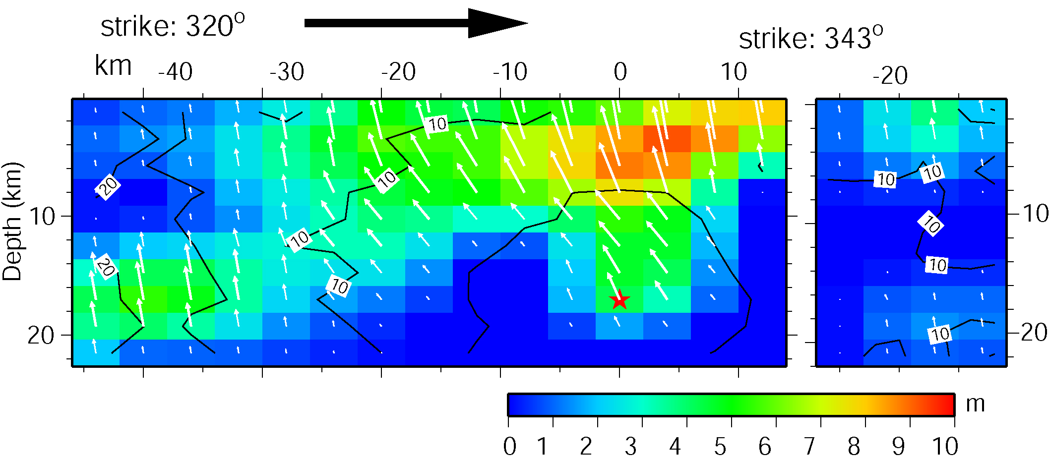
Figure: The big black arrow shows the fault's strike. The colors show the slip amplitude and white arrows indicate the direction of motion of the hanging wall relative to the footwall. Contours show the rupture initiation time and the red star indicates the hypocenter location.
Comparison of data and synthetic seismograms
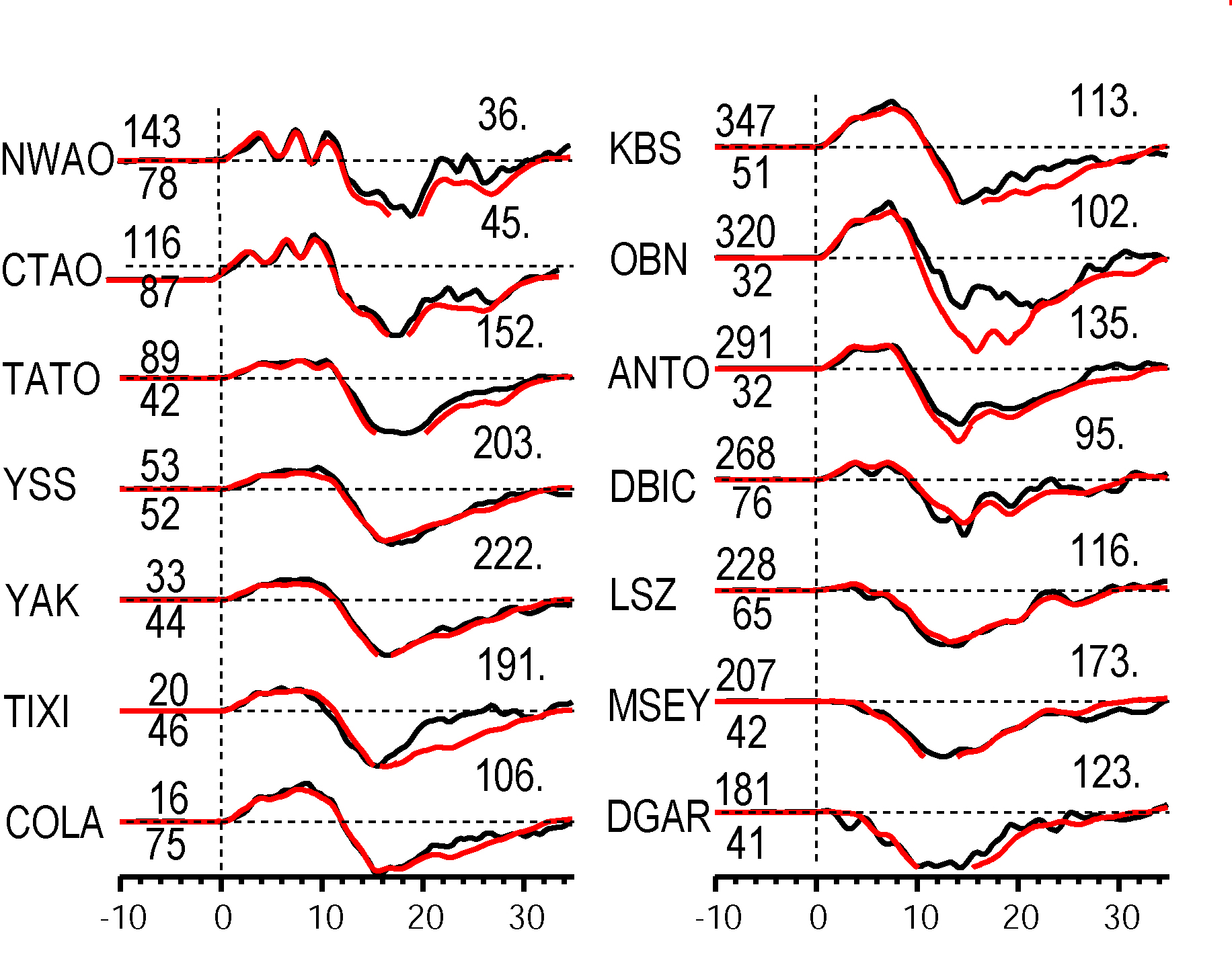
Figure: The Data are shown in black and the synthetic seismograms are plotted in red. Both data and synthetic seismograms are aligned on the P arrivals. The number at the end of each trace is the peak amplitude of the observation in micro-meter. The number above the beginning of each trace is the source azimuth and below it is the epicentral distance.
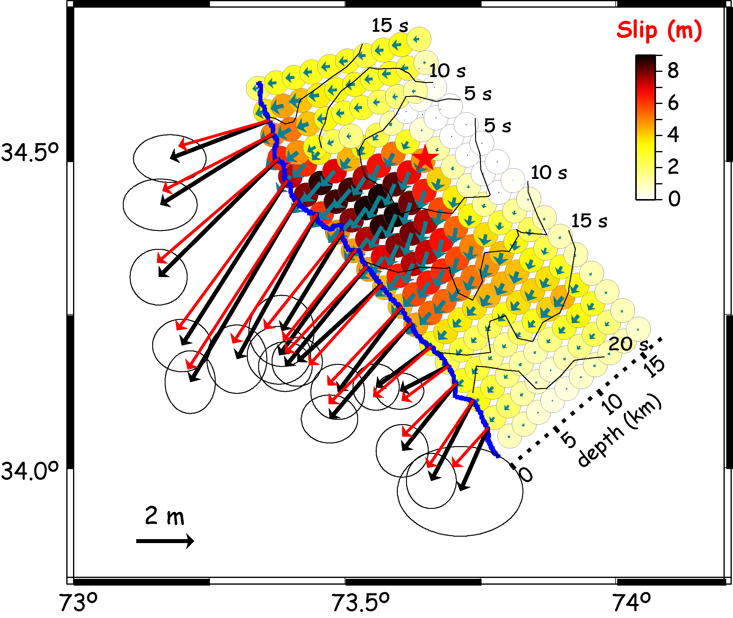
Figure: Surface projection of the slip distribution. The surface break obtained from geodesy is shown with black line. The measured surface offsets (black) and fits to these offsets from constrained seismic inversiona(red) are also shown.
Comments:
The SH waveforms were too broad to be used in the inversion. However, they were used to constrain the dip angle.
Download
(Slip Distribution)| SUBFAULT FORMAT | CMTSOLUTION FORMAT | SOURCE TIME FUNCTION |
References
Ji, C., D.J. Wald, and D.V. Helmberger, Source description of the 1999 Hector
Mine, California earthquake; Part I: Wavelet domain inversion theory and resolution
analysis,
Bassin, C., Laske, G. and Masters, G., The Current Limits of Resolution for
Surface Wave Tomography in North America, EOS Trans AGU, 81, F897, 2000.
Avouac, J. P., F. Ayoub, S. Leprince, A. O. Konca, and D. V. Helmberger,
The 2005, Mw 7.6 Kashmir earthquake: sub-pixel correlation of ASTER images and seismic waveforms analysis, Earth And Planetary Science Letters, 2006.
GCMT project: http://www.globalcmt.org/
USGS National Earthquake Information Center: http://neic.usgs.gov
Global Seismographic Network (GSN) is a cooperative scientific facility operated jointly by the Incorporated Research Institutions for Seismology (IRIS), the United States Geological Survey (USGS), and the National Science Foundation (NSF).
‹Back to Slip Maps for Recent Large Earthquakes home page