Updated Result
07/08/15 (Mw 8.0) , Peru Earthquake
A. Sladen, Caltech
DATA Process and Inversion
This is an update of our preliminary analysis based on the results published in Sladen et al. (2010). The source model is obtained by joint inversion of 6 InSAR images (ALOS tracks 109-110-111, ERS track 447, and Envisat wide-swath tracks 311 and 447), and 37 GSN broadband teleseismic body waveforms (22 P and 15 SH). We process the wide-swath images using the GAMMA™ software, and ROI_PAC for all the other images. The teleseismic data are downloaded from IRIS and converted into displacement by removing the instrument response. We use the epicenter of the USGS (Lon.=76.509° Lat.=-13.354°). The fault geometry is made of 3 planar segments of increasing dip angle (6,20 and 30°) to adjust the slab curvature. The segments are parallel to the trench with a 318° strike angle.Result
Cross-section of slip distribution
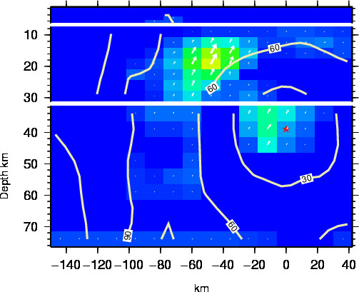
Figure 1: The colors show the slip amplitude and white arrows indicate the direction of motion of the hanging wall relative to the footwall. Contours show the rupture initiation time in seconds and the red star indicates the hypocenter location.
Comparison of data and synthetic seismograms
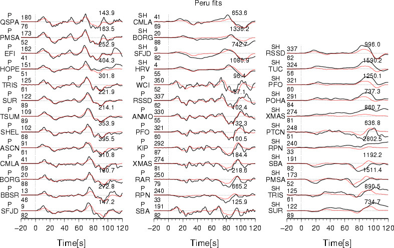
Figure 2: The Data are shown in black and the synthetic seismograms are plotted in red. Both data and synthetic seismograms are aligned on the P arrivals. The number at the end of each trace is the peak amplitude of the observation in micro-meter. The number above the beginning of each trace is the source azimuth and below it is the epicentral distance.
InSAR data and model residuals
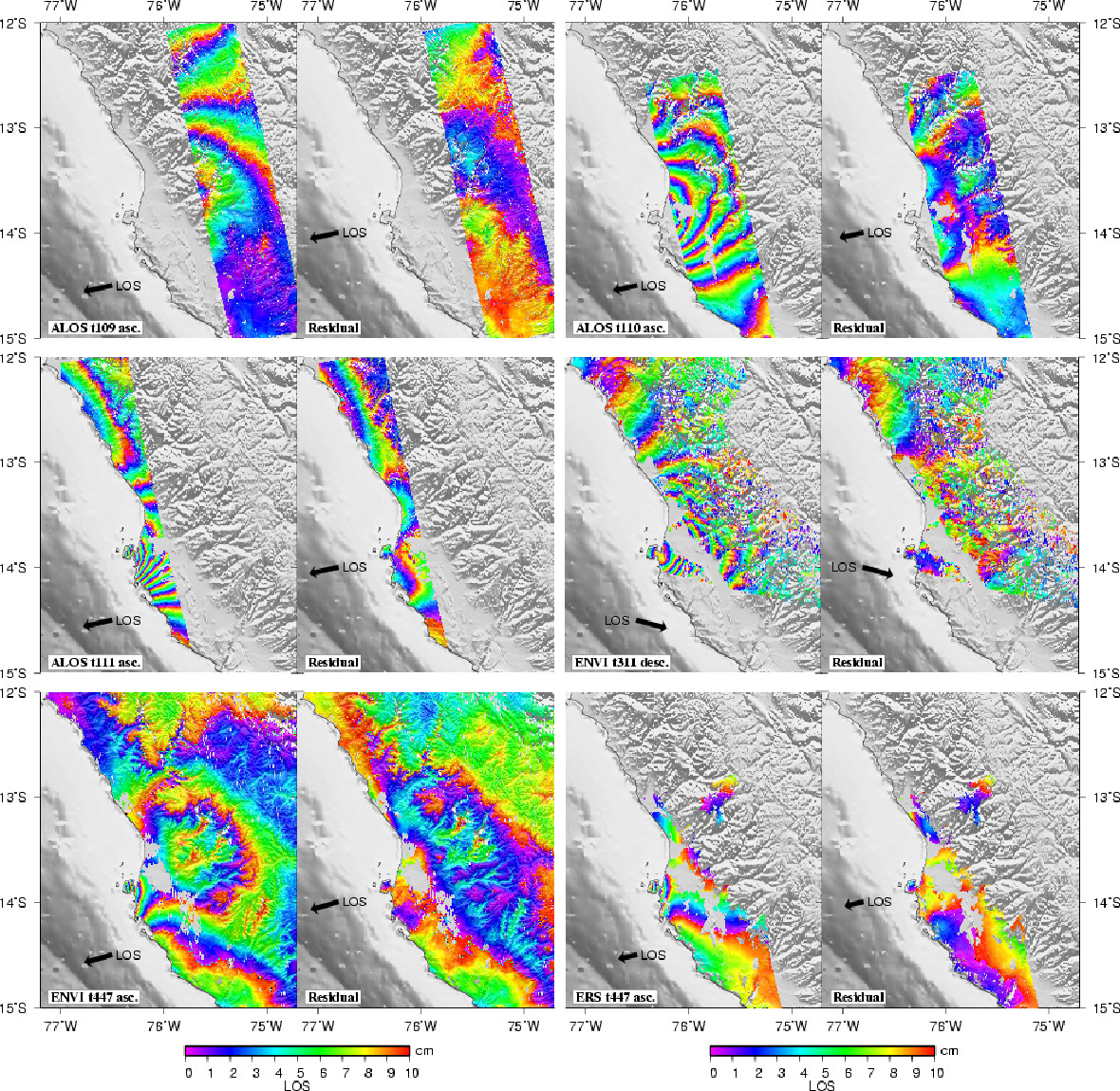
Figure 3: the 6 InSAR images used in the inversion and the residuals obtained by removing the model prediction and a linear ramp correction. All images are rewrapped at a 10 cm rate.
Map view of the slip distribution
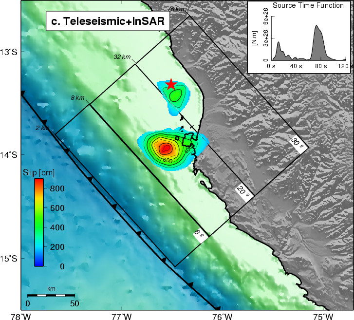
Figure 4: Surface projection of the slip distribution with contours in centimeters. The 3 black rectangles correspond to the segments of increasing dip angle which define the fault geometry. The inset shows the distribution of moment as a function of time during the rupture.
Comments:
Download
(Slip Distribution)| SUBFAULT FORMAT | CMTSOLUTION FORMAT | SOURCE TIME FUNCTION |
References
Bassin, C., Laske, G. and Masters, G., The Current Limits of Resolution for Surface Wave Tomography in North America, EOS Trans AGU, 81, F897, 2000.Ji, C., D.J. Wald, and D.V. Helmberger, Source description of the 1999 Hector Mine, California earthquake; Part I: Wavelet domain inversion theory and resolution analysis,
Sladen, A., H. Tavera, M. Simons, J. P. Avouac, A. O. Konca, H. Perfettini, L. Audin, E. J. Fielding, F. Ortega, and R. Cavagnoud, (2010), Source model of the 2007 Mw 8.0 Pisco, Peru earthquake: Implications for seismogenic behavior of subduction megathrusts,
GCMT project: http://www.globalcmt.org/
USGS National Earthquake Information Center: http://neic.usgs.gov
Global Seismographic Network (GSN) is a cooperative scientific facility operated jointly by the Incorporated Research Institutions for Seismology (IRIS), the United States Geological Survey (USGS), and the National Science Foundation (NSF).
‹Back to Slip Maps for Recent Large Earthquakes home page
© 2004 Tectonics Observatory :: California
Institute of Technology :: all rights reserved